Time Series Data In Pandas: An Introduction

Time series data measures something at a point or points in time.

• Stock prices or cryptocurrency values change over time, and finance data in general is often time series.
• Smart home devices are constantly monitoring what is going in your home and keeping track of various events to know when to turn on the lights or do whatever other task you've assigned it.
• Ride sharing apps like Uber and Lyft track their drivers to tell you how long a ride takes, how far away the driver is from you, etc.
• Security camera apps track events and can show you things like time-lapse.
• Server logs can be used to monitor when various events occur and can be used for analytics purposes or to discover security breaches.

The list goes on, but a lot of things that are tracked will have some kind of time stamp that is attached.

Time is important, and you can think about it in a few ways that are represented in Pandas.

1. Single moments in time, represented by time stamps.
2. Periods or intervals of time.
3. Differences in time - durations or time deltas.

In this post we will examine working with all of these representations with NYC 311 noise complaints data.

311 Noise Complaints

I'm looking at noise complaints specifically, but all 311 complaints have at least one timestamp, which marks when the complaint was created.

This data can be found here on NYC Open Data.

NYC Open Data API

I have this script that you can run to fetch the data from the NYC Open Data API - find it here.

To get an API key, check out this post.

If you run that script, you will end up with a Pandas DataFrame of the results, in the df variable.

df.head()

       borough           city              closed_date   ...   incident_zip resolution_action_updated_date  status
0  BROOKLYN     BROOKLYN       2019-01-01T02:22:46.000   ...    11231        2019-01-01T02:22:46.000        Closed
1  QUEENS       FRESH MEADOWS  2019-01-01T02:21:44.000   ...    11365        2019-01-01T02:21:44.000        Closed
2  MANHATTAN    NEW YORK       2019-01-02T02:07:11.000   ...    10003        2019-01-02T02:07:11.000        Closed
3  QUEENS       OZONE PARK     2019-01-01T07:01:51.000   ...    11417        2019-01-01T07:01:51.000        Closed
4  Unspecified  NaN            2019-07-29T12:17:22.000   ...    NaN          NaN                            Closed

[5 rows x 9 columns]

I only retrieved a subset of the columns because there are like 40-50 and most aren't relevant for this post.

df.columns

Index(['borough', 'city', 'closed_date', 'complaint_type', 'created_date', 'descriptor', 'incident_zip',
       'resolution_action_updated_date', 'status'],
      dtype='object')

There are three date columns in this dataset.

• created_date - this is when the complaint was created, whether someone called it in or submitted it online.
• closed_date - this is when the complaint was closed out in the system.
• resolution_action_updated_date - this is when there was an update with a resolution to the complaint, which could be when someone responded to investigate the complaint.

Dates in Python: the built-in datetime module

If you've worked with the datetime module in Python, you might be familiar with some basic operations.

from datetime import datetime,timedelta

We're looking at datetime objects which represent a particular date/time, and also timedelta which represents a duration, and then we will see their equivalents in Pandas.

A couple of datetime basics

Create a date.

date = datetime(2020,7,19)

Now use timedelta to calculate the date 365 days prior.

approximately_one_year_ago = date- timedelta(365)

Which gives you a new datetime.datetime object.

approximately_one_year_ago

datetime.datetime(2019, 7, 20, 0, 0)

Or subtract two dates to get a datetime.timedelta.

datetime(2009,1,1) - datetime(2008,1,1)

datetime.timedelta(366)

Working with dates in Pandas is similar.

Dates in Pandas: Time stamps

The Pandas equivalent of datetime.datetime is TimeStamp.

In Pandas the dates are stored using the NumPy datetime64 data type.

We can convert the complaints data columns to datetime format, using pandas.to_datetime().

A single column can be converted like this:

df['created_date'] = pd.to_datetime(df['created_date'])

In many cases, Pandas is smart and can parse the date format and figure out how to convert it - similar to the 3rd party dateutil package, which you can use to easily parse dates in almost any format.

We can use pandas.DataFrame.apply() and convert all three of the columns at once.

df[['created_date','closed_date','resolution_action_updated_date']] = df[['created_date','closed_date','resolution_action_updated_date']].apply(pd.to_datetime)

Setting a datetime index

We are mainly going to focus on the created date of the complaints, so now let's set that column as a DatetimeIndex.

df = df.set_index(pd.DatetimeIndex(df['created_date']))

With time series data, it's helpful to index the data by a datetime field.

Once you set a datetime index, you can easily do a lot of slicing and grouping of the data.

Slice the data between two dates

date_one = datetime(2019,5,1)
date_two = datetime(2019,8,1)

df[date_one:date_two].head()


                       borough      city         closed_date   ...   incident_zip resolution_action_updated_date  status
created_date                                                   ...                                                      
2019-05-01 00:00:00  BROOKLYN   BROOKLYN 2019-05-03 01:45:00   ...    11226       2019-05-03 01:45:00             Closed
2019-05-01 00:00:56  MANHATTAN  NEW YORK 2019-05-01 04:16:53   ...    10016       2019-05-01 04:16:53             Closed
2019-05-01 00:01:24  MANHATTAN  NEW YORK 2019-05-01 01:44:21   ...    10021       2019-05-01 01:44:21             Closed
2019-05-01 00:01:27  BROOKLYN   BROOKLYN 2019-05-01 00:43:11   ...    11216       2019-05-01 00:43:11             Closed
2019-05-01 00:03:55  BROOKLYN   BROOKLYN 2019-05-01 00:43:11   ...    11216       2019-05-01 00:43:11             Closed

[5 rows x 9 columns]

Date ranges and frequencies

In Pandas you have a lot of options whether you want to generate a date range, or group your data by some time-based frequency.

Generate a date range

You can generate a date range with pd.date_range().

At its most basic, just pass a start and end date, and it will return a DatetimeIndex.

pd.date_range('2019-07-05', '2019-08-20')

DatetimeIndex(['2019-07-05', '2019-07-06', '2019-07-07', '2019-07-08', '2019-07-09', '2019-07-10', '2019-07-11',
               '2019-07-12', '2019-07-13', '2019-07-14', '2019-07-15', '2019-07-16', '2019-07-17', '2019-07-18',
               '2019-07-19', '2019-07-20', '2019-07-21', '2019-07-22', '2019-07-23', '2019-07-24', '2019-07-25',
               '2019-07-26', '2019-07-27', '2019-07-28', '2019-07-29', '2019-07-30', '2019-07-31', '2019-08-01',
               '2019-08-02', '2019-08-03', '2019-08-04', '2019-08-05', '2019-08-06', '2019-08-07', '2019-08-08',
               '2019-08-09', '2019-08-10', '2019-08-11', '2019-08-12', '2019-08-13', '2019-08-14', '2019-08-15',
               '2019-08-16', '2019-08-17', '2019-08-18', '2019-08-19', '2019-08-20'],
              dtype='datetime64[ns]', freq='D')

You can also provide only a start date and then specify the number of periods you want, along with the frequency, which defaults to days, which you can see in the basic example output above.

In the next example I've supplied a starting date, specified 10 periods, with an hourly('T') frequency.

pd.date_range('2019-07-05', periods=10, freq='T')

DatetimeIndex(['2019-07-05 00:00:00', '2019-07-05 00:01:00', '2019-07-05 00:02:00', '2019-07-05 00:03:00',
               '2019-07-05 00:04:00', '2019-07-05 00:05:00', '2019-07-05 00:06:00', '2019-07-05 00:07:00',
               '2019-07-05 00:08:00', '2019-07-05 00:09:00'],
              dtype='datetime64[ns]', freq='T')

Date offsets and frequencies

Pandas offers a number of frequencies and date offsets with aliases like 'B' for business day, or 'MS' for the first calendar day of the month.

The aliases can also be combined, which we will look at in a bit as well.

• Find all of them here in the docs.

Resampling

You might want to convert frequencies, such as from days to weeks, minutes to seconds, etc.

There are a few ways you might want to convert the frequency.

• Converting one equal frequency to another.
• Downsampling, or converting higher to lower frequency, such as from days to weeks.
• Upsampling, or converting lower to higher frequency, such as from weeks to days.

Upsampling and handling missing values

When upsampling, you can provide a method to fill in missing values, for example filling forward or backwards.

If you don't specify a method, it will just leave the missing values as NA.

• Read more on handling missing values in Pandas here.

Converting frequencies with asfreq()

If you are converting from one frequency to another and they are equal frequencies, you can just use the asfreq() method.

This method mostly generates a date range for the new frequency and calls reindex - read more in the docs.

It returns a selection of the original data - the value at the end of each frequency interval - with its new index.

The index needs to be unique.

df.index.is_unique

False

That's not really surprising because there are probably multiple complaints created at the same time.

For demonstration purposes, I'm just going to drop duplicates.

df = df[~df.index.duplicated(keep='first')]

Then convert to a daily frequency.

df.asfreq('D')

If you're looking to use aggregate functions on the new groups, then you will probably want to use resample() instead, since asfreq() returns the last value in each frequency group as opposed to something like the mean or count.

Grouping time series data and converting between frequencies with resample()

The resample() method is similar to Pandas DataFrame.groupby but for time series data.

You can group by some time frequency such as days, weeks, business quarters, etc, and then apply an aggregate function to the groups.

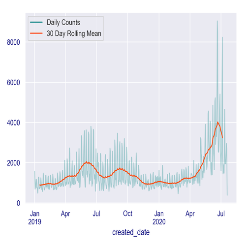
The daily count of created 311 complaints

df.resample('D').count() 

Weekly counts.

df.resample('W').count()

The weekly frequency defaults to splitting up weeks on Sunday, but maybe you want to split the weeks up on another day like Wednesday.

df.resample('W-WED').count()

The 311 noise complaints could be grouped by 8 hour periods.

df.resample('8H').count()

There are a lot of options, and the offsets can be combined as well, like here we group them by 8 hours and 30 minutes instead of 8 hours.

 df.resample('8H30T').count()

Financial data

If you're working with financial data, you can group by quarterly data, or only on business days, and so forth.

Periods and intervals in Pandas

Next we look at the Pandas Period, which represents non-overlapping periods of time, and has a corresponding PeriodIndex.

Since periods are non-overlapping, each time stamp can only belong to a single period for a given frequency.

You can generate a range of time periods in a similar way to how we generated a date range earlier, with pd.period_range(), specifying the number of periods and the frequency.

pd.period_range('2015', periods=8, freq='Y')

PeriodIndex(['2015', '2016', '2017', '2018', '2019', '2020', '2021', '2022'], dtype='period[A-DEC]', freq='A-DEC')

Here I generated 8 year periods from 2015.

Converting a DatetimeIndex to a PeriodIndex

Use the to_period() method to convert a DatetimeIndex to a PeriodIndex, and just specify a frequency.

Here we convert with a daily frequency, but you can customize this like we did with the DatetimeIndex.

df.to_period(freq='D')

And the new index looks like this:

PeriodIndex(['2019-07-10', '2019-07-10', '2019-07-10', '2019-07-10', '2019-07-10', '2019-07-10', '2019-07-10',
             '2019-07-10', '2019-07-10', '2019-07-10',
             ...
             '2019-08-17', '2019-08-17', '2019-08-17', '2019-08-17', '2019-08-17', '2019-08-17', '2019-08-17',
             '2019-08-17', '2019-08-17', '2019-08-17'],
            dtype='period[D]', name='created_date', length=48516, freq='D')

Duration: time deltas in Pandas

Time deltas represent a duration of time, or a difference in time.

We saw the example at the beginning of the post of calculating the date one year ago with a time delta, or subtracting two datetime objects to get the duration between them.

Pandas has a Timedelta object, which is a subclass of datetime.timedelta and is based on NumPy's timedelta64 data structure.

You can convert data from a recognized time delta format to a Timedelta object with pd.to_timedelta().

There is an associated TimedeltaIndex as well.

To generate a TimedeltaIndex, you can use pd.timedelta_range().

Here I'm generating a time delta range from a 1-hour duration to a 5-hour duration with an hourly frequency.

pd.timedelta_range('1 hour', periods=5,freq='H') 

• Check out the docs for more on parsing timedeltas and how to format them - Pandas is smart and can parse many different formats, like in this example I just used the string '1 hour'.

Here is the TimedeltaIndex that was generated.

TimedeltaIndex(['01:00:00', '02:00:00', '03:00:00', '04:00:00', '05:00:00'], dtype='timedelta64[ns]', freq='H')

Duration between when 311 complaints are opened and closed

With the 311 data, we might want to look at the time duration between when a complaint was opened and then closed.

Noise complaints are supposed to be responded to within 8 hours, so it could be interesting to look at the response time.

If we just subtract the created date(which we set as the index earlier) from the closed_date, the resulting data type is timedelta64.

df['duration'] = df.closed_date - df.index

Here I created a new column duration with the result.

df.duration.head()

created_date
2019-07-10 00:00:07   02:47:31
2019-07-10 00:00:18   03:41:05
2019-07-10 00:00:21   03:25:42
2019-07-10 00:01:00   02:05:06
2019-07-10 00:01:23   07:15:02
Name: duration, dtype: timedelta64[ns]

And you can see that the datatype is timedelta64.

You could set the duration column as the index.

df.set_index(pd.TimedeltaIndex(df['duration']))

Which gives you a TimedeltaIndex.

TimedeltaIndex(['0 days 02:47:31', '0 days 03:41:05', '0 days 03:25:42', '0 days 02:05:06', '0 days 07:15:02',
                '0 days 00:15:25', '0 days 01:45:03', '0 days 06:33:36', '0 days 00:52:52', '0 days 00:21:31',
                ...
                '0 days 01:56:54', '0 days 15:46:43', '0 days 01:47:48', '0 days 01:04:48', '0 days 01:22:12',
                '0 days 04:45:00', '0 days 02:02:09', '1 days 03:08:04', '0 days 00:04:57', '1 days 02:41:48'],
               dtype='timedelta64[ns]', length=48516, freq=None)

Shifting data

Shifting is another common manipulation with time series data with some interesting uses.

• Calculate return on investment (ROI) of a stock.
• Lag features in machine learning - shift the data and use past values as features.

Shifting can be very useful to calculate differences over time when you shift the data by a certain amount and then make comparisons.

With 311 complaints data, maybe the NYC government is trying to predict how many complaints they are likely to get in the future so that they can have enough agents working to handle the volume.

One or more lag features might be used to train a model to predict future complaint volume.

It could also be helpful to look at complaints now compared to a year ago or some other time period to examine possible trends.

There are two ways to shift data with Pandas.

Shift the data with shift()

First we will shift the data 90 days.

daily_counts = df.resample('D')['complaint_type'].count()
daily_counts.shift(90)

See the difference in these plots.

The green line is at July 1, 2019.

Since the data moves, you can see that the line has shifted 90 days to October.

Shift the index with tshift()

Next we will shift the index.

daily_counts.tshift(90)

And compare the plots below.

You can see how the index shifted 90 days to starting at April.

Rolling window calculations

Calculating something like a rolling mean or average is good when analyzing longer term trends in the data and smoothing out short-term fluctuations that might just be noise.

How does it work?

• Takes a specified window size, like 30 days.
• Makes calculations such as the mean on the data in that window.
• Then it rolls or steps over the rest of the data, making the calculation on the window sized data chunk at each step.

You can calculate rolling means and other rolling window calculations with DataFrame.rolling.

I'm going to use the daily counts and take a rolling average of the mean, with a window size of 30 days.

daily_counts = df.resample('D')['complaint_type'].count()
rolling = daily_counts.rolling(30)

Thanks for reading!

Now you're ready to get started working with time series data in Pandas.

Let me know if you have any questions or comments, and if you're working on any interesting projects!

Leave a comment or reach out to me on Twitter @LVNGD.